Background knowledge: Energy Time Curve (ETC)
Target Audience
All who have a certain technical scientific interest and have already read the chapter Background knowledge. Anyone who would like to understand the relationship between reflections and impulse response in more detail.
Reflexionen finden
Use in YouTube ⚙ Subtitles for videos in German language.
The ETC (Energy Time Curve, also Impulse Response Envelope) is calculated from the impulse response. More precisely, the Hilbert Transform is meant here. Other providers use the term for the logarithm of the squared impulse response (Log-Squared-ETC). The latter does not have its own name in Hifi apps, it is output in the "Logarithmic" / [RAW] view.
The ETC should highlight the maxima due to reflections more clearly than the raw data by suppressing other maxima. From the distance between the peaks of direct sound and reflection, the detour of the reflection can be read in meters - as in the case of ground reflection in geometrical acoustics. After that you can use the "string method" to find the reflecting surface. To do this, you stretch a string between the microphone and the loudspeaker (in case of doubt the midrange or tweeter) and then extend it by this detour. If you find a surface that a) would reflect the loudspeaker if it were made of glass and b) can be touched with the stretched string at the reflection point (with a tolerance of 10 or 20 cm), then this surface is most likely the cause of the reflection.
In the next step, damping material can be applied there on a trial basis and checked to see whether the sound and measured values improve. In case of doubt, the thickness of the damping material should not be spared: Narrow displayed peaks are particularly conspicuous in the measurement data, but technically they are only caused by the reflection of the highest frequencies. Thin damping material makes them disappear in the output, with the superficially friendlier measured values the sound may even deteriorate [Zehner]. Suppliers of damping material specify the respective frequency range for their products. If you are not familiar with the material, you should insulate at least down to 1 kHz, better still much lower. Before ordering, the area can be insulated on a trial basis with clothing or bedding. Rule of thumb: for some effect down to 1 kHz, the latter should have a thickness of $\lambda/4\simeq 10 $cm, thicker would certainly be better.
ETC alone is not a magic formula for displaying reflections, so the following sections are intended to provide an overview of the technical background and the optimal interaction with smoothing and other displays.
Pressure and velocity
A resonance can be imagined as an interaction between back-and-forth motion (velocity) and pressure of the air. This is very simple with waves which do not propagate, e.g. with this room mode:

In the center of the image there is maximum velocity while the pressure hardly changes. At the edge of the image, the opposite is true.
The energy is alternately in the kinetic energy of the air in the center of the room and in the pressure difference between the areas near the walls.
In the case of a propagating wave that spreads out from the sound source, this interaction is somewhat more complicated, but this does not change the basic idea.
Now one could assume that in the case of a reflection the sound arrives from the source with a time delay and that therefore each peak or larger deflection in the impulse response corresponds to a reflection. If by chance several reflections had the same detour and thus the same propagation delay (e.g. at wall and floor), this would be easy to control with different microphone positions. In fact, this method sometimes works quite well, there is only one fundamental problem: As soon as the sound excites a resonance in the room (actually always), an oscillation is generated which can be seen as such in the impulse response (see numerous pictures at Measurements).
The impulse response is also zero, where this oscillation has zero crossings. And by the wave character maxima and a minima arise around it. Usually one works with the logarithmized amount - there several maxima would show up, which hardly differ from closely spaced real reflections. In practice this makes it problematic to distinguish, for example, whether several separate peaks indicate a single reflection or several independent reflections [Zehner].
A proposed solution was published in [Heyser 1971]. Both our ear and common microphones react only to the pressure part of the wave, velocity receivers are hardly used. This can ultimately lead to the misleading results: If there is silence at a certain measurement location for a certain frequency, it can mean that a) there really is no sound energy there, or b) most of the energy is in the velocity, such as in the middle of the animation above. The measured and audible sound pressure is highest there at the right and left edges.
The measured and displayed impulse response thus contains "only the directly relevant, audible half" of the physical energy. Intuitively it is clear that the "other half", i.e. the velocity is just as important: If it were zero in the middle of the animation, there would be no sound pressure at the edge. Heyser starts with energy conservation for all Fourier components of the wave and completes the missing part with a mathematical trick (see below). As a result, correlated sound components are smoothed, while singular ones keep their shape. The "waves" are lost, the reflections remain. The physical sound energy is not reflected by this, it is not evenly distributed in a propagating wave. The aim of the method is rather to smooth out coherent ripples by resonances, leaving incoherent disturbances by reflections unaffected. According to Heyser, the ETC should not be viewed as an envelope, but rather as the full, complex analytical signal. The following pictures show some strengths and weaknesses of this approach.
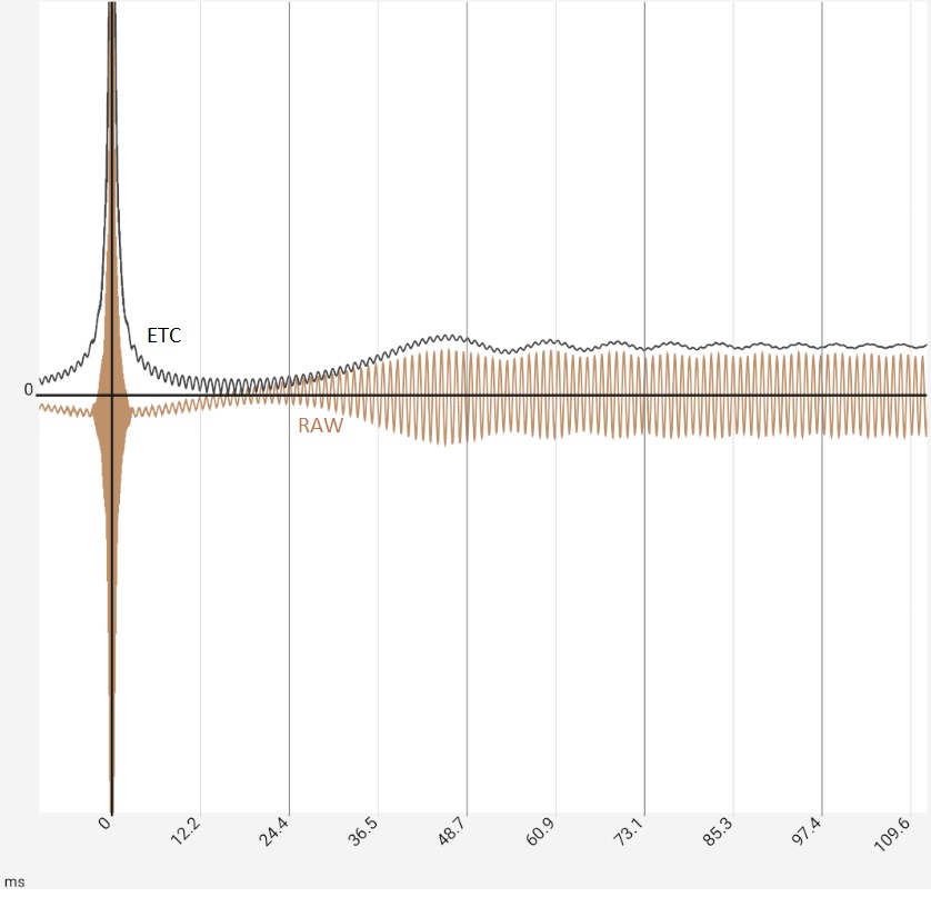
The basis are 3 log sweeps, which were added time-shifted via wave editor. These were "simulated" to the app as a microphone signal. This is to simulate the direct sound of a loudspeaker and two delayed events. The reflections are 2 ms apart in each case, which corresponds to 0.68 and 1.37 m of additional distance, e.g. a reflection on a wall and on the floor. The first logsweep was left unprocessed, the two reflected logsweeps were clipped at 1 kHz with 12 dB/octave. In practice, this could be caused by a carpet or foam in a piece of furniture. The goal is to detect the two reflections as reliably as possible anyway.
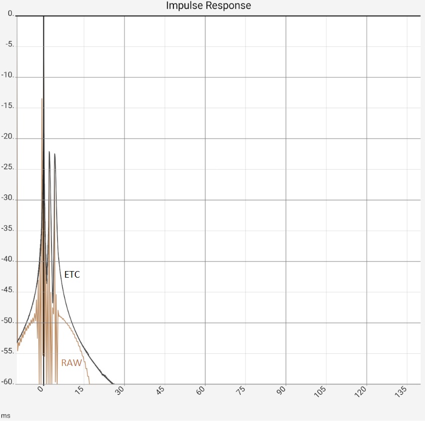
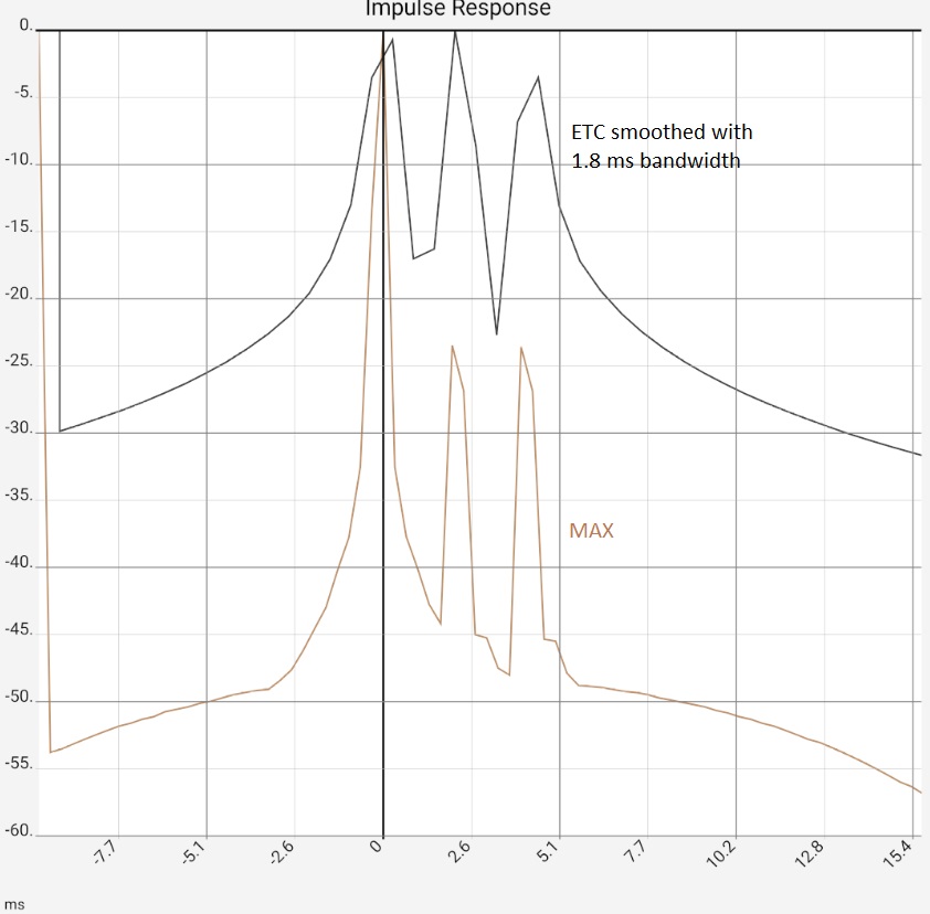
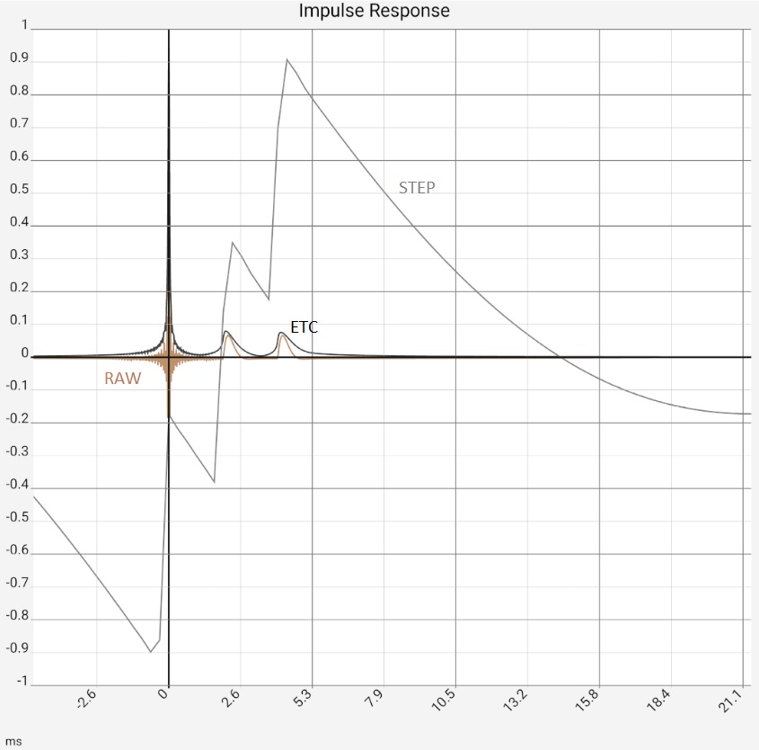
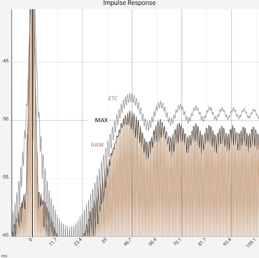
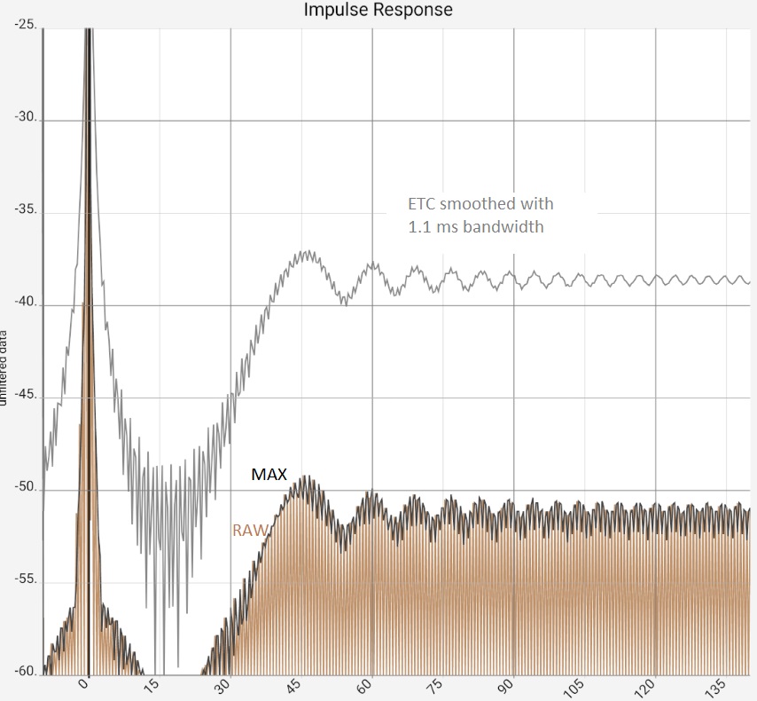
The first image represents the situation after program start, in practice the two peaks would typically be somewhat higher at -10...-20 dB due to the reflections, as they contained more higher frequency components and would thus be correspondingly more "peak-like". Figure 2: After zooming in and switching from raw data [RAW] to maximum values [MAX] it would be clear "that there is something there". The ETC works out the peaks but does not bring any new insights compared to switching to [MAX]: The app then only shows the maximum values (of 0.5 ms sections) of the impulse response. The steps in the brown curve are caused by the interaction of resolution and zoom, i.e. they are a technical artifact. Completely smoothed, on the other hand, is the high-frequency oscillation around the first peak. This is caused by the limiting of the frequency response (see below), but this is also the same with [MAX]. In the third image, the ETC has been additionally smoothed, flattening the first peak at 0 accordingly. Since the maximum remains fixed at 0 dB, the two reflections now stand out clearly. The last image shows the same data in linear representation. The two reflections are now easy to miss in the raw data because they have lost their "peakedness" due to the missing high frequency components. The reflections are best worked out by the STEP curve, which is calculated from the integral of the raw data. The area under the small humps due to the reflections is comparable to the one under the first peak.
| Impulse response | Zoom to initial area | With smoothing | Linear representation |
| Click images to enlarge | |||
 |
 |
 |
 |
|
Column 1: Raw data (brown) vs. ETC Column 2: Zoom view of the first image, for the raw data switched to MAX to hide the fluctuations. Column 3: In addition to Figure 2, ETC curves were smoothed with 0.9 ms bandwidth. The increase in the peaks is primarily due to a reduction in the maximum: This is always fixed at 0 dB. Column 4: Linear plot: raw data (brown) vs. ETC (black) and step response (gray) | |||
So in this case the ETC brings practically no insights, smoothing or [STEP] function are the better way. The opposite picture shows up, if the microphone signal is replaced by a logsweep (2 sec, 20 Hz - 20 kHz), to which additionally (from approx. 1.1 sec) a 1 kHz signal with the same level was added. The latter is supposed to represent the extreme case of a resonance, perhaps caused by a ventilation duct:
| Impulse response | Zoom to initial area | Logarithmic representation | With smoothing |
| Click images to enlarge | |||
 |
 |
 |
 |
|
Column 1: Linear plot of raw data (brown) vs. ETC Column 2: Zoom view of the first image. Column 3: In addition to Figure 2, ETC curves were smoothed with 0.9 ms bandwidth. The increase in peaks is primarily due to a reduction in the maximum: This is always fixed at 0 dB. Column 4: Linear plot: raw data (brown) vs. ETC (black) and step response (gray) | |||
Fig. 1 and 2: This is where the ETC can show its capabilities: The 1 kHz signal (brown) can be optimally captured due to the high coherence and is almost completely smoothed (gray). Fig. 3: Logarithmization and maximum value generation also fail to deliver a comparable result. Figure 4: With some anticipation of which frequencies will be reflected, an appropriate smoothing for ETC can additionally be selected. This again improves the quality of the ETC output data. Filtering the signal, e.g. with a low-pass filter at 2 kHz provides similar results in this example, but could allow further improvements in practice.
In practice, the ETC is used by some sound engineers as an important aspect for more certainty in the interpretation of measured reflections. A real gain can only be expected in interaction with filtering, smoothing and other representations.
Technical background
Heyser starts with energy conservation for all Fourier components of the wave, so, graphically speaking, he adds a cos term for the velocity to the sinusoidal progression of the pressure so that the total energy remains constant because of $\sin^2x + \cos^2x = 1$. This achieves a uniform energy density over the wave train of each Fourier component and eliminates disturbing zero crossings in the impulse response. In practice, one obtains such a situation e.g. in Kundt's dust tube, a propagating wave has no uniform energy density. The ETC therefore does not represent the real, measurable energy density.
The calculation is illustrated here with an artificially produced impulse response: The microphone signal was replaced by a log sweep (2 sec, 20 Hz - 20 kHz), to which a 1 kHz signal with the same level was added (from approx. 1.1 sec).
![]()
1: The 1 kHz signal can be seen in the impulse response (after 40 dB amplification) and represents the misunderstood reflection: Each maximum is similar to a reflection and thus complicates the interpretation.
2: The frequency response is calculated by Fourier transformation, the peaks at 1 kHz are clearly recognisable in the real and imaginary parts. Since the impulse response was real-valued, the real and imaginary parts (even and odd) are mirror symmetrical.
3. So no information is lost when the right-hand part is removed. Viewed graphically, however, the respective mirrored term $\exp(-i\omega t)$ is lost in the Fourier space for each $\exp(i\omega t)$, so that instead of $\sin$ or $\cos$ terms, $\exp(i\phi)$ terms whose magnitude is constant now appear in the reverse transformation. If one enlarges the result, a corresponding picture emerges:
4. In the last step, the reverse transformation takes place. The new terms now create an imaginary part, the app outputs the absolute value as the result. In the enlargement you can see that the FWHM of the peak widens by 2 samples due to the added imaginary part: In step 1, the peak is 1 sample wide, followed by brief high-frequency filter clanking because the sweep ends at 20 kHz. At step 4 the FWHM is 3 samples. Nevertheless, it can be said that no resolution is lost by the operation: the widening is 2 samples, i.e. its physical value in ms is 0.042 ms at 48000 samples/s, or 0.01 ms at 192k, or 3 mm sound propagation time. So it is an artifact of the limited resolution and not a problem of the method.
![]()
A zoom on the result (step 4) shows: real and imaginary parts are out of phase in $\pi/2$, the magnitude is constant enough not to be interpreted as reflection.
References
[Heyser 1971] Heyser, Richard: Determination of Loudspeaker Signal Arrival Times - Part III. J. Audio Eng. Soc. 19, 902 (1971). Abgedruckt in "An anthology of the works of Richard C. Heyser on measurement, analysis, and perception" AES - Time Delay Spectroscopy, Seite 44ff, 57ff
[Zehner] Markus Zehner: "Messungen und Interpretation von ETCs / Reflektierte Fehlschlüsse" www.zehner.ch/lab/etc.html, www.zehner.ch/lab.html