Calibration of the built-in microphone on Android devices
Background knowledge
Microphone calibration requires a great amount of experience and makes up the majority of the more than 300-page book [Handbook of Condenser Microphones] or the dissertation [Bouaoua], for example. In Germany, the Physikalisch-Technische Bundesanstalt (PTB) researches and develops methods for this. In order to achieve reproducible results with verifiable accuracy for home use, at least the following must be taken into account:
- "Microphone" here always means pressure microphone; "measurement microphones" are assumed to have an omnidirectional characteristic.
- Any microphone (even omnidirectional) may react differently depending on the directionaldistribution of the incident sound [IEC 61094-7], [Walber].
A distinction is made between
- Calibration by Free-Field Response (the sound comes from an almost point source from a defined direction, reflections are negligible. A so-called free-field microphone has been calibrated in this way, with sound coming from the front, and should also be used in this way).
- Random Incidence and Diffuse-Field Calibration (the sound comes "from everywhere" due to reflections on the walls)
- Pressure Calibration (This method is used in manufacturing [Wikipedia]. The microphone is placed in a closed container for this purpose. Known pressure changes are generated in it, e.g. by a motor-moved piston or an electrostatic actuator).
- In connection with this, there are different technical procedures [Nedzelnitsky], [Wikipedia]. Here used is the comparison calibration:
 Statement StatementIn some discussions, measurements with the built-in mobile phone microphone are dismissed as a "gimmick", whereas a measurement microphone is associated with "professionalism". This is a rather emotional statement; the decisive factor is which requirements have to be met: For example, in comparative measurements between different listening positions, the (relative) differences often play a much greater role than the (absolute) accuracy of the values. The measured reverberation time also hardly depends on the microphone used. Although the frequency response of the built-in microphone is not linear, it generally has no "dents" below 4000 Hz that are typical for room acoustics. In other words, such dents are definitely caused by the room and not by the microphone. Many important room acoustic effects can therefore be recognised. After the calibration with home tools described here, the frequency response and the directional dependence of the mobile phone microphone are also known well enough to gain insights for further decisions from the measurement results.
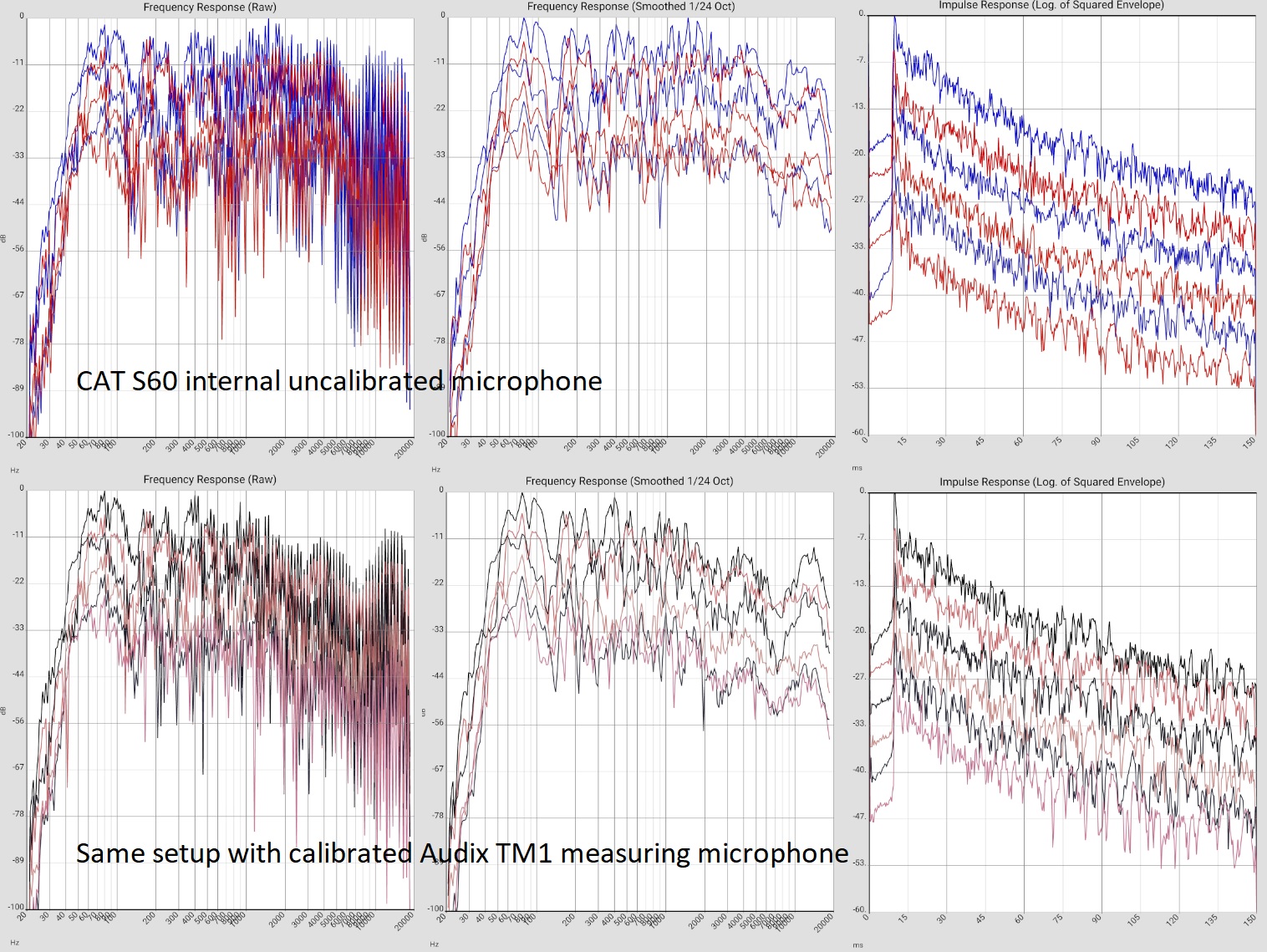
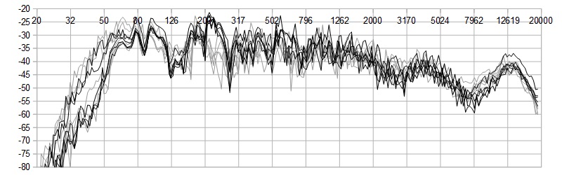
The illustration shows an example of the comparison of the frequency response and impulse response of two Martin Logan Classic ESL 9 loudspeakers at different listening positions in a room with above-average damping.
The upper curves are measured with the uncalibrated microphone of a CAT S60 mobile phone, the lower ones with a calibrated measuring microphone:
You can see how much more important the interaction between the loudspeaker and the room is for the results than the microphone in question. (Of course, this should by no means lead to the conclusion that every measurement is possible with mobile phone microphones).
|
Before you start
My first tests with cell phone microphones showed extreme bass drop, which is not to be expected even with an uncalibrated microphone. The reason is easy to find if you convert an old headset into a "loopback" circuit, i.e. feed the output signal directly into the microphone input.: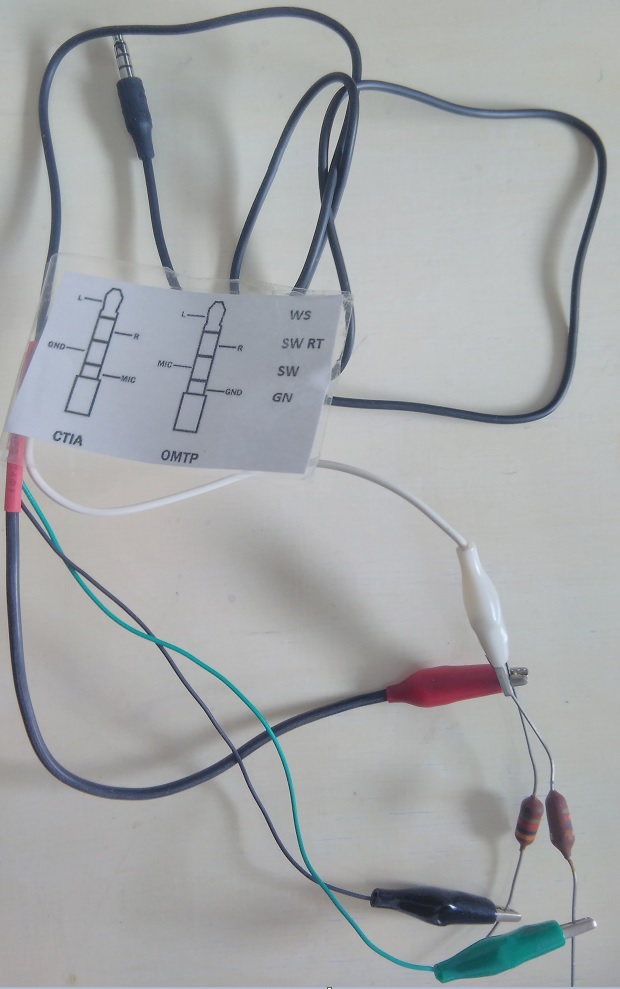
Loopback circuit for Android devices with 3.5mm jack. The circuit loops the headphone signal back to the microphone input. The 3k resistors seem to be (also) necessary for the phone to switch to "external microphone". The frequency response can then be measured with hifi apps via logsweep. See also https://source.android.com/devices/audio/latency/loopback
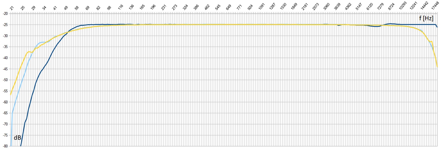 Frequency response measured via loopback with Hifi Apps. Yellow, blue: Lenovo P10400, black: CAT S60. Logsweep 20 Hz - 20 kHz, 2 sec, yellow curve only 15 Hz - 20 kHz, 10 sec.
The frequency response of the "pure device" without microphone drops sharply in the bass range, perhaps to suppress wind noise during phone calls. The drop above 10 kHz in the Lenovo tablet is less important in the later assessment: Treble losses in need of correction due to "muffled" rooms start earlier and are also easily perceptible without measurement.
Hifi apps allow you to store a corresponding file in addition to the calibration files of the microphones for correction. It is important that these corrections are also necessary for an externally connected measurement microphone when the headphone jack is used. When using an external converter via USB, they do not matter. Fortunately, the 16 bit sampling depth of the signal offers a lot of reserves for corrections: Mathematically 20 * log(2^16) = 96 dB dynamic range, of which 40 or 50 dB are certainly still usable in practice. The uppermost 20 dB are omitted because some devices perform a dynamic compression at high sound pressure, the lowest 20 dB are omitted due to quantization noise and noise of the electronics in the device, furthermore the modulation is subject to a certain uncertainty during the measurement.
Some smartphones use several microphones to separate ambient noise from the useful signal during conversations. This electronic processing is counterproductive for measurements, so Hifi apps access the raw signal of the microphone. Since it cannot be guaranteed that every device handles this access correctly, several options for audio input can be selected in the setup.
Diffuse-Field Calibration with Household Remedies
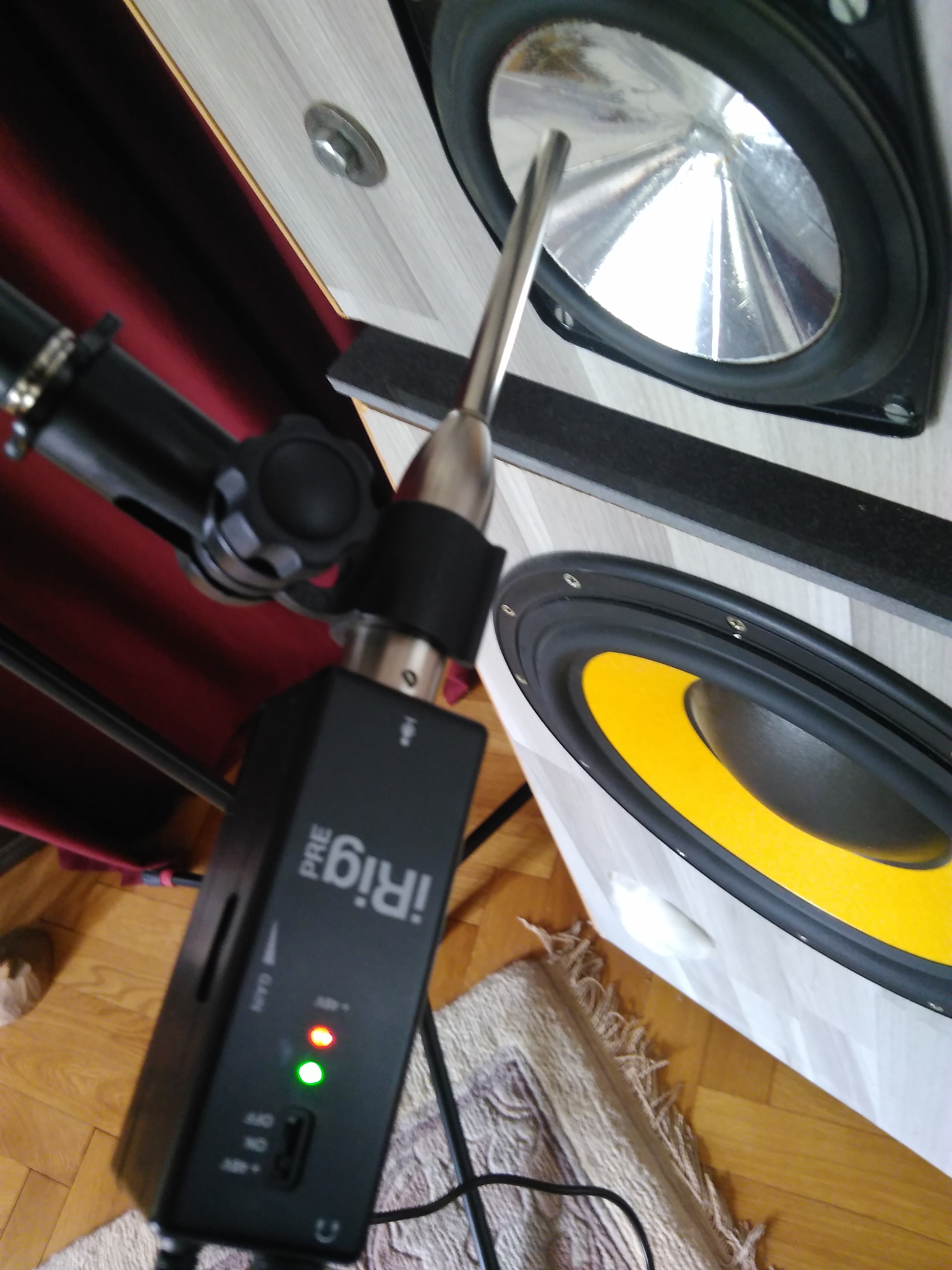
The apps offer the option to calibrate the internal microphone of the Android device against a measurement microphone. In addition to a (borrowed) measuring microphone, this requires an amplifier with two speakers in an average living room. The entire procedure takes about 20 minutes:
- If there is a file with calibration data for the measurement microphone, set up the microphone in the app.
- Connect the Android device to the measurement microphone.
- Connect the Android device to the amplifier and stand at a listening position equidistant from both speakers to measure.
- Make one measurement each with the measurement microphone and the internal microphone under otherwise as identical conditions as possible.
- If you are satisfied with the measurements, now select "Microphone Calibration" and there your two measurements.
- Hifi-Apps calculates the calibration curve from the difference.
What accuracy can be expected?
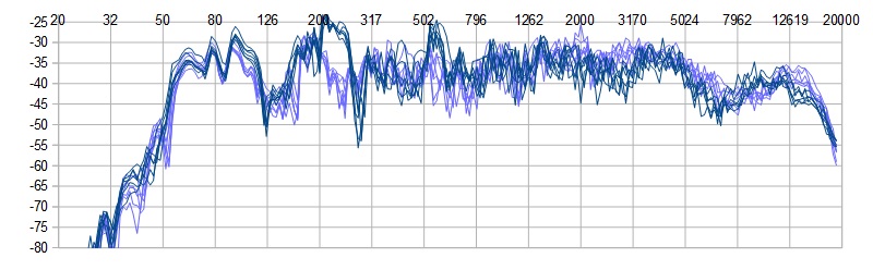
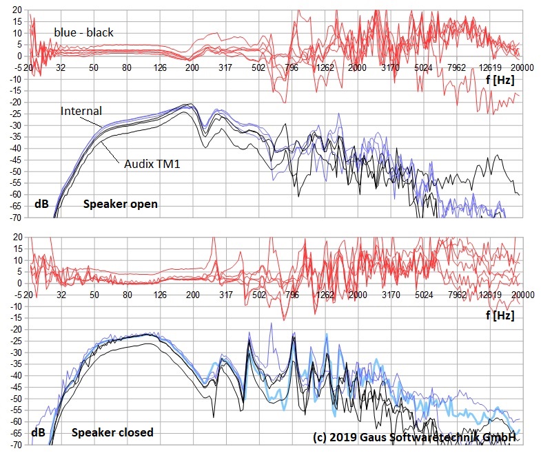
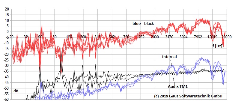
The following pictures show the measured frequency response at the listening position in a well-damped room as an example. The blue curves were recorded with the uncalibrated internal microphone of a CAT S60 cell phone, the black ones with an Audix TM1 measurement microphone. The microphone was moved 10 cm forward, backward, sideways and upward respectively, hence the different curves. The two brightness levels represent the two stereo channels. The red curve shows the calibration curve of the CAT microphone, it was determined by near field recording.In one of the two speakers, the damping material was removed from the midrange enclosure to simulate a slight defect. The frequency responses therefore diverge clearly at around 200 to 300 Hz and visibly at the first harmonic around 500 Hz. The defect is even more noticeable in the cell phone measurement, presumably because the direct sound component is somewhat larger due to the directional characteristic. The measurement microphone reacts more sensitively to the room influences.
Automated interpretation of hifi apps would provide the following information for both microphones:
- Channel uniformity problems in the 200 to 300 Hz range
- Ripple in the bass range is acceptable, room resonances are below 10 dB. This shows that comprehensive damping measures have already been taken, more is not necessary.
- Cancellation at 126 Hz, perhaps a floor bounce. More precise would be calculated by comparison with measurements at other places.
- Frequency response in the midrange acceptable
- Additional information from the impulse response (not shown here) about the reverberation characteristics of the room.
- Also not shown here are comb filter effects, from which, together with the impulse response, conclusions can be drawn about the LEV. can be drawn.
- Suggestions for setting an equalizer up to about 5 kHz.
- Safe information about the range below 40 Hz.
- Dip at 7 kHz (intentional, de-esser). This is also visible when recording with an uncalibrated microphone, but it could also be an artifact of the microphone. A calibrated cell phone microphone also reacts too sensitively to the position of the cell phone housing in this case.
- Treble drop. The loudspeakers have plasma tweeters radiating all around, whose frequency response drops considerably more in all measurements than the listening impression would suggest. In general, no linearity is to be expected at the listening position, but rather a drop of a few dB from about 5 kHz, Similar to a distant lightning only the low rumble of thunder remains audible. This effect is generally referred to as dispersion.
- Suggestions for setting treble controls, if the speakers have any.
- Suggestions for setting an equalizer over the entire frequency range.
- Comparability with other systems, thus more exchange of experience between experimenters.
The decade from 200-2000 Hz, which is important for speech transmission, is reproduced very well in all devices reviewed.
The deviations here are better than in the CAT S60 in most cases, often even in the 2 dB range.
Up to 5 kHz it remains "still quite decent" in all cases:
The sensitivity sometimes increases, but remains (almost) monotonous. In the range above that, considerable fluctuations are possible.
With the uncalibrated Android microphone, a "good-natured" curve can be expected in the range from 50 Hz to 5 kHz, i.e. within an arbitrarily selected octave, the fluctuations will be limited to a corridor of +/- 3dB width.
|
Directional characteristic For room measurements, measuring microphones with omnidirectional characteristics are usually used. The cell phone microphone, on the other hand, has a directional characteristic. During telephone calls, it should pick up as little ambient noise as possible. As a result, reflections from the walls are weighted less heavily. Various test series have shown that slightly turning sideways in order to "as skillfully as possible" capture part of the room reflections does not provide reproducible results. The device must be pointed in the direction of the listener's gaze for each measurement. In the end, the direct sound from the loudspeakers is evaluated somewhat more strongly, which makes it impossible to compare measurements from different devices. Measurements with the same device can of course be compared. |
Estimation of uncertainties
In this chapter, the systematic and statistical errors in the calibration according to the above recipe are estimated. Without error estimation, the measurement results would not be usable.
|
Note Please remember that even a measurement microphone may have changed its characteristics over the years. In the private sector, regular recalibrations as under laboratory conditions are certainly not appropriate. However, an occasional comparison measurement with a (borrowed) second measurement microphone or the reproduction of an old measurement cannot do any harm. Otherwise, you run the risk of producing incorrect measurement results for years without noticing it. |
Measurement in the diffuse field of a living room is subject to the "curse of many parameters". Changes of the microphone position by a few cm lead to strongly different results. The main reason is the interaction of the different reflections. This makes averaging and/or processing of the results with certain smoothing algorithms necessary.
To ensure that the results processed in this way are not only "glossed over" but also useful for calibration, they are compared here with measurements in the free field and pressure measurements. With well defined ratios the conversion of the methods into each other is possible with accuracies of less than 1 dB [Milhomem], [Jacketta].
The guiding principle was to find sound sources whose frequency response over a few octaves a) does not exhibit any visible comb filter effects due to reflections without any smoothing and b) does not depend on small changes in the position of the microphone. In these ranges, the results measured by cell phone and measurement microphone were compared so that the differences in the frequency responses for free field and pressure could be compiled. These were then compared in turn with the results of the recipe described above.
For the low frequency range a so-called Linkwitz dipole was used. This could optionally be closed by placing a sealed plate on the sound outlet. This made two series of measurements possible: one at the open system in the mouth to imitate a free field, the other in the closed system. The former seems possible for the bass range because the wavelengths considered are considerably larger than the sound exit aperture. Thus, one can assume that the airflow there is relatively uniform. Likewise, there should be uniform pressure in the closed system due to the long wavelength in the bass range. These theses were verified by at least six, often considerably more measurements with different microphone positions.
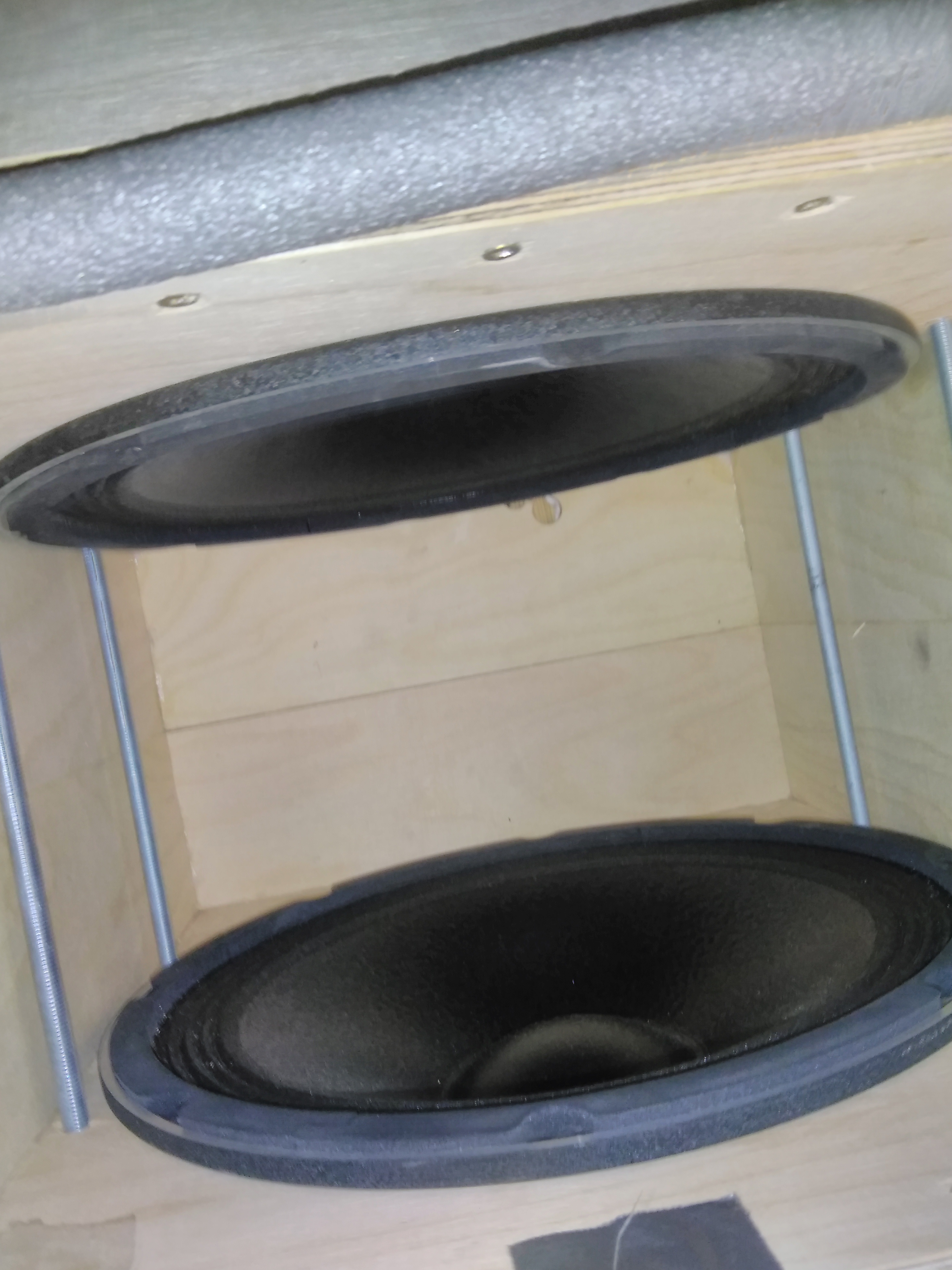
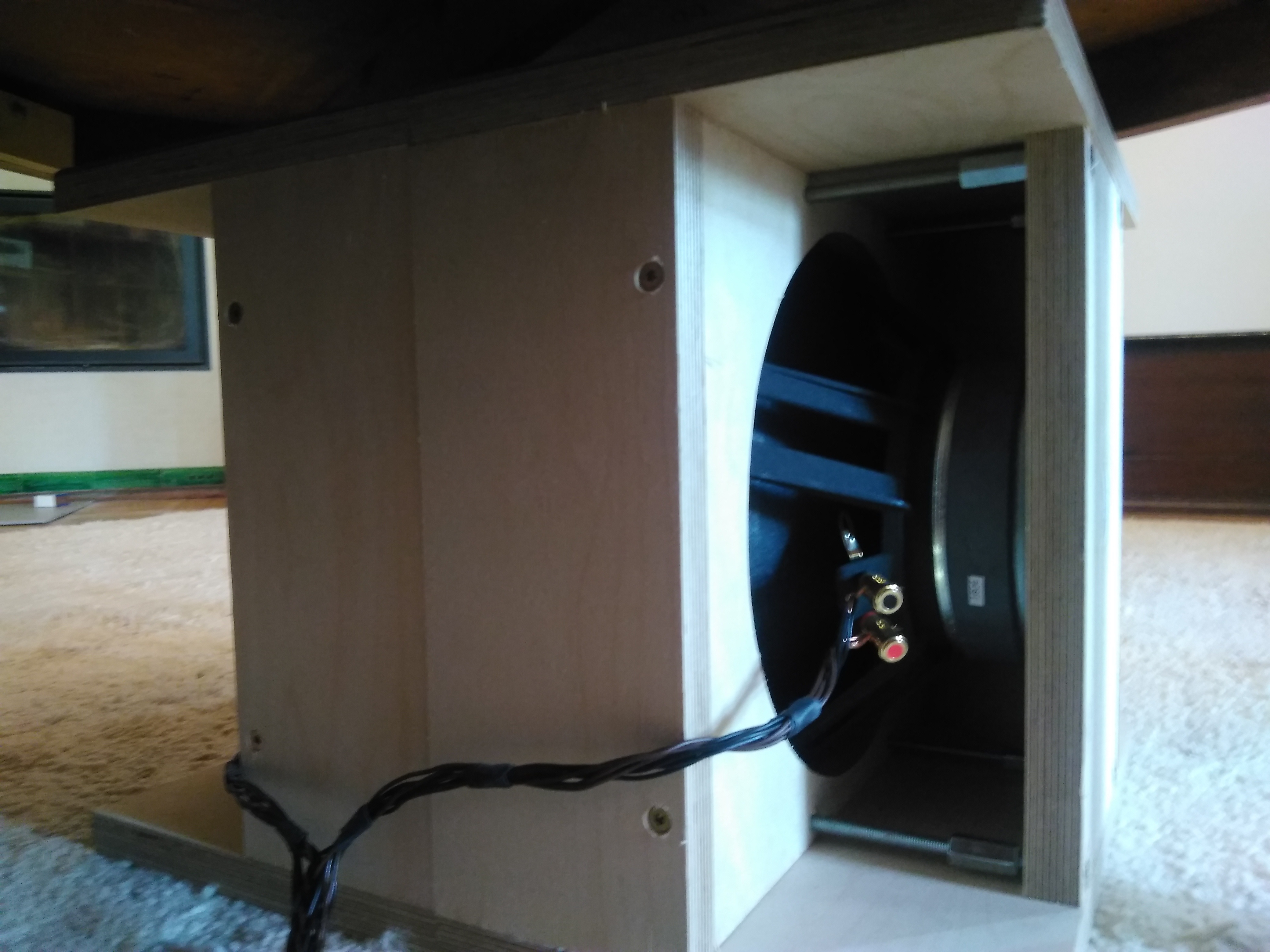
Linkwitz dipole with two 30 cm IMG Stage Line SP-12A/302PA chassis. In the middle there is enough space for a cell phone.
Comparison of the frequency responses of an internal cell phone microphone with a measurement microphone inside the housing of a Linkwitz dipole. The red curves show the differences in dB.
To simulate a free field in the midrange an Expolinear Görlich midrange driver was used. The particularly stiff sandwich diaphragm used in this chassis should generate as uniform a wave field as possible to simulate a free field.
Expolinear Görlich TT 130 G bass-midrange driver which was connected via a voltage divider to a Lamm 1.2 Reference power amplifier. The cabinet was a block of solid concrete with a tube about 34 cm long and 12 cm in diameter.
In the high-frequency range, some experiments were initially started in the near-field of various large-area electrostats, magnetostats, ribbons and air-motion transformers, the results of which were all disappointing. Apparently, a free point source is a better choice. Therefore, the tests were continued with different plasma tweeters. Plasma tweeters work without mechanical parts by ionizing the air, i.e. the near field is not distorted by wave propagation in a vibrating medium. In fact, the frequency response and impulse response were much clearer than with other tweeters.
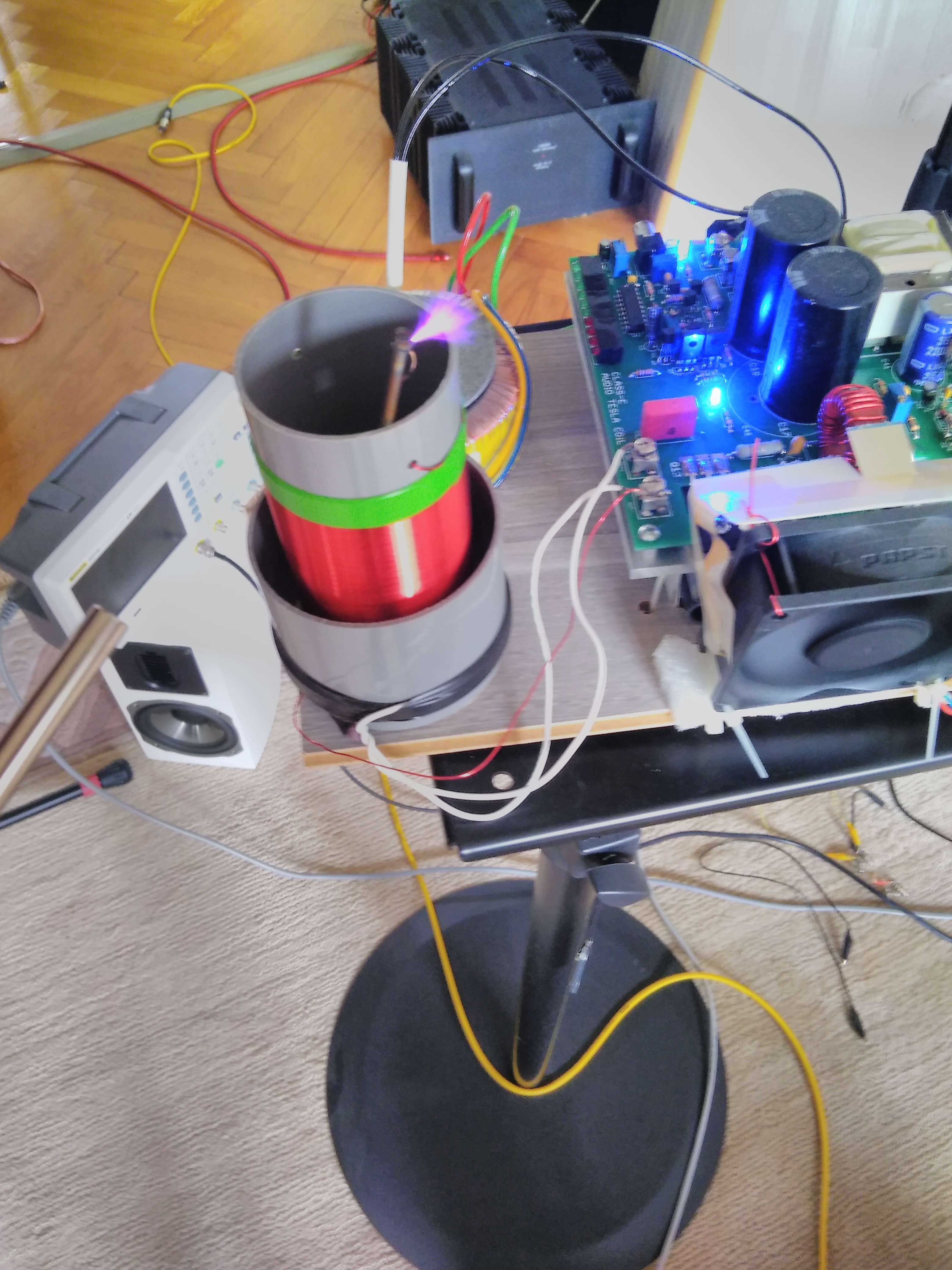
Broadband plasma loudspeaker as an almost ideal point source of sound for the range above 2000 Hz. Slightly above the center of the image, the violet glowing discharge is visible. The music frequency is modulated onto the 4 MHz carrier. The loudspeakers cannot be used for listening to music because of the low sound level and the discharge noise, However, when played on a test basis, they produce an impressive localization and stage.
Result
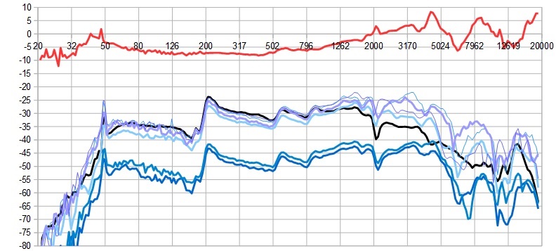
If the ranges of the various near-field measurements are added together, the following picture emerges for the calibration curve:
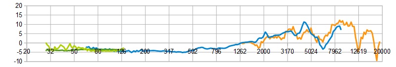
The light green and dark green curves are data from the closed and open Linkwitz dipole, respectively, the blue curve was measured in the near field of the Görlich midrange driver and the brown curve is from measurements at the plasma tweeter.
In the range from 80 to approx. 4000 Hz, the significant errors of the cell phone microphone are recorded similarly by all measurements. The curves increase by about 10 dB in this range. The deviation of the curves from each other, on the other hand, is considerably lower. Below 80 Hz, the accuracy decreases. The range above 4000 Hz is, as discussed above, not reliable enough for measurements. It should only be used for orientation, e.g. to generate targeted listening tests.
In the range up to 4000 Hz, the curve is very smooth overall. In this respect, it seems appropriate to also smooth the curves recorded at the listening position with an octave bandwidth.
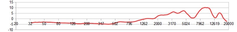
If the overlapping areas of the combined curves are averaged and the result is smoothed with an octave bandwidth, the following picture is obtained together with the values measured at the listening position:
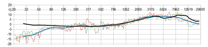
The black curve is the result of the merged nearfield measurements, the thin curves in red and green are recorded at the listening position according to the above recipe. Their mean value smoothed over one octave is shown in blue. From 200 Hz up to about 4000 Hz an excellent agreement is noticeable - the deviations are in the range of 1 or 2 dB. The fluctuations of the unsmoothed curves seem to compensate each other. Since it cannot be assumed that this is always the case, the error is estimated very conservatively in the "Conclusion" box.
|
Fazit Near-field measurements show that the frequency response of the cell phone microphone from 80 to about 4000 Hz is not linear but quite "good-natured": No fluctuations appear that could be misunderstood as room effects in need of correction: The fluctuations are a maximum of 5 dB per octave and 10 dB over all values, mostly considerably less. Below 80 Hz, the frequency response is linear enough to still reliably detect the typical room effects in need of correction with bandwidths below one octave and amplitudes above 10 dB. However, a quantitative evaluation is not possible. Above 4000 Hz, the frequency response of the built-in microphone is no longer reliable despite correction. Calibration at the listening position according to the above recipe reduces this uncertainty considerably. If deviations of 10 dB or more are still detected in the frequency range mentioned with a microphone calibrated in this way, this is no longer attributable to the microphone. A measuring microphone will then detect similar deviations. |
Literatur
[ARTA] ARTA Chamber for the Lower End Microphone Calibration http://www.artalabs.hr/AppNotes/AP5_MikroMeasChamber-Rev03Eng.pdf[Bouaoua] Nourreddine Bouaoua: Free-field Reciprocity Calibration of Condenser Microphones in the Low Ultrasonic Frequency Range, Dissertation 2007 https://d-nb.info/989266540/34]
[faberacoustical] iPhone 4 Audio and Frequency Response Limitations http://blog.faberacoustical.com/2010/ios/iphone/iphone-4-audio-and-frequency-response-limitations/
[Frederiksen] E. Frederiksen, Acoustic metrology – an overview of calibration methodsand their uncertainties Int. J. Metrol. Qual. Eng.4, 97–107 (2013) https://www.metrology-journal.org/articles/ijmqe/pdf/2013/02/ijmqe130045.pdf
[Handbook of Condenser Microphones] AIP Handbook of Condenser Microphones: Theory… (Hardcover) by George S.K. Wong, Tony F.W. Embleton
[hifi-selbstbau.de] Mikrofonkalibrierung, wie geht das? 2013 https://www.hifi-selbstbau.de/grundlagen-mainmenu-35/softwaremesstechnik-mainmenu-66/100-mikrofonkalibrierung-wie-geht-das
IEC 61094-4, “Specifications for Working Standard Microphones,” International Electrotechnical Commission, 1995.
IEC 61094-5, “Methods for pressure calibration of working standard microphones by comparison,” International Electrotechnical Commission, 2001.
[IEC 61094-7] Measurement microphones, Part 7: Values for the difference between free-field and pressure sensitivity levels of laboratory standard microphones
IEC 61094-8, “Methods for determining the free-field sensitivity of working standard microphones by comparison,” International Electrotechnical Commission, 2012.
[Jacketta] Implementation of a diffuse-field microphone calibration system
Richard J Jacketta, Conference Paper inter.noise 2012
[Krump] Akustische Messmöglichkeiten mit Smartphones Gerhard Krump DAGA 2012 - Darmstadt
[Milhomem] Electroacoustics and Audio Engineering: Paper ICA2016-147 An investigation ondiffuse-field calibration of measurement microphones by the reciprocity technique Thiago Antônio B. Milhomem(a), Zemar Martins D. Soares(b), Ricardo Eduardo Musafir(c) PROCEEDINGS of the 22ndInternational Congress on Acoustics ICA 2016 [Nedzelnitsky] Laboratory Microphone Calibration Methos at the National Institute of Standards and Technology, U.S.A. https://www.nist.gov/sites/default/files/documents/calibrations/aip-ch8.pdf
[technical-direct] Smartphone User Experience Analysis – Audio (II) 2016 http://www.technical-direct.com/en/smartphone-user-experience-analysis-audio-ii/
[Tipton] DIY Microphone Calibration By Ron Tipton http://www.tdl-tech.com/miccalax.pdf
[Ossietzky] https://d-nb.info/989266540/34 Free-field Reciprocity Calibration of Condenser Microphones in the LowUltrasonic Frequency Range Von der Fakultät für Mathematik und Naturwissenschaftender Carl von Ossietzky Universität Oldenburgzur Erlangung des Grades und Titels eines Doktors der Naturwissenschaften (Dr. rer. nat.)angenommene Dissertation von Nourreddine BOUAOUA Geboren am 15. Dezember 1975in Algier (Algerien)
[Walber] https://www.audioxpress.com/article/acoustic-methods-of-microphone-calibration Acoustic Methods of Microphone Calibration by Chad Walber This article was originally published in Voice Coil, September 2017.
[Wikipedia] https://en.wikipedia.org/wiki/Measurement_microphone_calibration