Background knowledge
Compared to the original literature, this is already an abridged version. It was precisely because of the extensive knowledge available that the idea was ultimately born to incorporate and automate some of it in Hifi-Apps - so that the user can perform the most important optimizations even without prior knowledge. So in this sense, the reading is optional. Enjoy.
Who is supposed to read all that?
All those who have a certain technical scientific interest and consequently do not want to use Hifi-Apps blindly. Everyone who knows that you can use a system better if you know what is happening "in the background". Anyone who uses Hifi-Apps in unusual situations and therefore needs to change the default settings.
Music reproduction - even with the highest quality equipment available - always differs significantly from the original. Here various physical effects are explained, which are responsible for this and how the knowledge about this is incorporated into hifi apps. This is not meant to spoil anyone's enjoyment of music at the highest possible level - what priority technical "waveform fidelity" has in the process varies greatly from person to person. However, if you enjoy constantly optimizing your system, you should not lose sight of this technical aspect.
The effects listed are limited to what Hifi-Apps can also measure. They are far from complete: Other cables, capacitors or tubes can create a completely new listening experience, although the measured values do not change significantly.
You should also keep in mind some basic limitations in music reproduction: No loudspeaker radiates directionally like the musical instrument being reproduced (trumpet to the front, violin to the top). The wave field of a concert hall cannot be reconstructed. Not even with many loudspeakers in surround systems and certainly not with the few channels of a common music recording.
Even if you limit yourself to a single listening position and correct the signal electronically (e.g. with FIR or IIR filters) the result is far from the original: The musical instruments have to be mapped to places where there is usually no loudspeaker. However, the generation of such phantom sound sources already yields different results depending on the recording method. Since the sound comes from the loudspeakers and not from the place where the phantom source should be, the localization will also change depending on frequency and head movement (keyword: Head-Related Transfer Function).
The conclusion is that current measurement methods can only partially represent what is heard and felt. In general, some readily measurable physical quantities are surprisingly unimportant to the listening experience during playback, while other clearly audible (and blind-test confirmed) characteristics are barely visible in measurements commonly used today. Current research in the field of psychoacoustics is investigating such relationships.
Hifi Apps builds on this insight: After the measurement, adapted test tones are generated for listening tests, so that the user can judge how important a found resonance, reflection, irregularity in the delay time, etc. really is for their hearing sensation.
Our Boundaries or: The Acoustic Curtain
In a thought experiment from the 1930s, the ideal system for music reproduction was conceived: An orchestra plays behind a soundproof wall into which holes are drilled bit by bit. The listeners hear the orchestra better and better - after a certain number of holes, it will sound like "without a wall" to everyone.
Now the holes are replaced by (imaginary) distortion-free microphone-recorder-loudspeaker combinations. The orchestra can now play time-shifted and you get the ideal reproduction.
Unfortunately, even this imaginary (in any case hardly realizable) setup does not reproduce the original 1:1. It would have to consist of many very small loudspeaker-microphone combinations. As soon as one starts from a technically realizable size (let's say a wall of the size 3 x 5 m with 1500 channels driving 10x10 cm loudspeakers), waves below the order of magnitude (here 10 cm or 3 kHz) are radiated according to the radiation characteristics of the chassis - the synthesis of the wave field according to the Huygens principle is thus disturbed and the thought experiment fails.
Where do Hifi-Apps come in?
Fortunately, there are physical quantities that are easily measurable and (usually) also have a strong influence on the listening experience. The best known example is probably the frequency response. The following sections explain all measurement variables used in hifi apps.
In the interaction of loudspeakers and listening room, reflections, resonances, etc. create various effects that can positively or negatively influence the listening experience. Hifi-Apps determines from the results of measurements and hearing tests which of these effects should be corrected and suggests improvements.
Different ranges of frequency response and reverberation time are responsible for completely different effects. The subdivision made here is based mainly on the articles by Toole and Griesinger cited below. The areas in which the different effects occur partly overlap.
Ultimately, however, there remains a margin of judgment in each case: Live recordings already contain the acoustic properties of the concert hall and studio recordings can be prepared in a comparable way. From this point of view, the listening room should not also "play into it", i.e. be as anechoic as possible, especially if these signals are added by surround systems anyway. On the other hand, certain room influences are desirable for more "live-ness". It has long been established that the absence of room reflections in normal stereo playback only produces a "flat frontal sound" [Griesinger 1999].
Hifi-Apps do not have the arrogance to pretend an "absolute truth" here. No evaluation takes place within the mentioned margin of judgment, and the margin itself can be changed in the setup. And the "last instance" is always the listening test.
Bass range up to ca. 150 Hz
The range below 20 Hz can be used in gaming or home theater for vibration effects. In Hifi-Apps the measurements start at 20 Hz or higher.
LFE vs. Subwoofer
The range up to approx. 120 Hz is sometimes (e.g. with 5.1-channel audio - Dolby Digital film) transmitted via a separate channel: Low-Frequency Effects (LFE). LFE is not the same as "subwoofer", but rather the LFE signal is mixed 10 dB higher, so that even with three front speakers and several surround speakers a tonal balance is achieved with their music signals [dolby.com What is the LFE channel?].
The usual subwoofer outputs of amplifiers can be controlled by the LFE signal and/or the low-frequency components of the remaining channels, but can also be switched off (in "Pure Direct" mode). The full stereo signal then goes directly to the right and left front speakers.
The crossover frequency and other parameters are usually set as low as the front speakers can (comfortably) handle, often 80 Hz at 12 dB slope. Before each measurement, it must therefore be ensured that the subwoofers are correctly driven: For most measurements, the subwoofers must be switched on. Exceptions are measurements to determine the transition parameters mentioned above.
A sound source with less than 80 Hz cannot be localised. However, this does not at all mean that the location of the subwoofers is indifferent. Firstly, at this transition frequency and e.g. at 12 dB octave slope, signals with 160 Hz are only attenuated by 12 dB (320 Hz corresponds to 24 dB), i.e. still clearly audible (10 dB less is subjectively "half as loud"), and sources with these frequencies are locatable. Flow noise in the bass reflex channel and harmonics due to distortion can also be added. Evolutionarily, the localisation of low frequencies was also important for our survival. Our hearing is capable of locating with very little usable information.
Secondly, in typical living rooms, the so-called room modes are excited in this range: the air in the listening room can resonate at certain frequencies, as shown in Fig. 1.

Fig. 1. The first room modes on a rectangular surface. In practice, the third dimension is added, as shown at [falstad]. The modes are most audible in the areas where the color concentration changes the most.
Our ear reacts to pressure, i.e. the modes are particularly audible in the range in which the number of particles fluctuates. The speed of the particles (velocity) is not audible. Common subwoofers (bass reflex) also generate pressure fluctuations, Velocity is generated by Linkwitz dipoles, for example.
Room modes are particularly annoying with long-lasting basses, as they become more and more resonant. But they also take away the dryness and precision of short basses: In the worst case, a hard-played kick bass can excite a room mode so much that the highest level becomes blurred in the listening impression or is even perceived later. Such spongy, boomy delays may be impressive at first thanks to their high volume, but the music loses its accentuation or "foot bounce factor" or "punch" as a result (especially at low volumes). Of course, it is not forbidden to enjoy this as "powerful bass" - the optimal listening room does not require the same sterility and neutrality as a recording studio. But then, in addition to the lack of punch, it should also be noted that our brains infer a small, confining space from sharp, widely spaced room modes. An organ concert will never sound airy and spacious as in a church when individual low notes build up. Experienced listeners, when asked for a judgment, will express more or less directly, depending on their character, that they associate inferior or improperly set-up equipment with this sound - no matter what was on the bill.
The first perception of room modes often happens through cancellations "hardly any bass despite powerful subwoofer". Later, irregularities in bass runs and a lack of precision become noticeable. Both subwoofers and listening positions should be positioned in such a way that individual room modes are not unnecessarily noticeable. Details about this can be found in [Olive 1995], [Bech 1998].
Intuitively, it seems obvious that narrowband room modes with a long decay time (technically: high $Q$) are particularly unpleasant. The prevailing opinion is that reducing this $Q$ leads to a more balanced sound image. However, this is not unreservedly correct [Toole and Olive (1988) ].
Hifi-Apps therefore only evaluate the deviations in frequency responses [Louden].
For "noticeable" peaks (with high Q and high amplitude) a targeted listening test is constructed so that the user can decide for themselves whether they already know the characteristic sound and whether they want to do something about it.
Berechnung vs. Realität
The room modes can be calculated analytically for cuboid-shaped rooms as in Fig. 1.
From the results it can be seen that particularly few pressure fluctuations occur in the middle of the room width and at 38% of the room length.
However, the "best possible" placement of subwoofers and listening positions according to this "38% rule" is only useful in practice on a trial basis.
For living rooms, there are too many factors that are difficult to assess:
The result is heavily altered by the installation location of subwoofer(s), damping, furnishing, doors and windows.
A quantitative determination of all these factors is hardly feasible.
Another approach for the placement of the loudspeakers is the "1/5 rule".
According to this, the membrane of the loudspeaker should be e.g. at 5 m room length (in the direction in which the loudspeaker radiates) 1 m in front of the wall. Sometimes the 2/5 rule is suggested, which is close to 38%. Or simply "at least 1 meter from the wall".
These are also useful approaches for a test run, but not universal recipes.
Theoretically, more complex spaces could also be calculated (with numerical methods).
However, this only makes sense for precisely defined mass products (e.g. combustion engines with associated exhaust system).
However, the calculated values for a cubic room can certainly be used for a first orientation:
If the longest distance between parallel walls is 4m / 5m / 6m, no room modes below about 34 Hz, 29 Hz, 24 Hz are to be expected.
(The acoustic size of a room is typically 10%-20% larger than its dimensions due to deflection of doors, windows and walls).
Ultimately, however, only the measured values and listening tests count.
Various authors [Peter 2013] have measured real listening rooms and compared the results with computer simulations, which are closely related to the models described above.
They also made their own comparisons between measurements and calculations.
The results can be summarised as follows:
The second point of the results was to be expected - otherwise the use of multiple subwoofers would be pointless.
Usable for hifi apps, on the other hand, is the knowledge about the orders of magnitude:
Based on the measured values, the user can be encouraged to move the loudspeakers, listening positions or damping elements by an appropriate amount in the most likely meaningful direction.
However, he must start a new measurement afterwards.
Suggestions for improvement based solely on an estimate of the result without measurement would be too unreliable.
A quantitative calculation of the listening room is not common even in the studio area. An interpretation of the calculated or measured results in the sense of "the peak at x Hz is due to room characteristic y" is only possible in rare cases.
Hifi apps are designed to take measurements at many points in the room one after the other. The position is determined automatically based on the sound travel times and the results are saved automatically. This makes it possible to create a frequency-dependent sound pressure map relatively quickly, from which you can directly see the behaviour of the room. Here is the sound pressure distribution of the same room at 140 Hz and 170 Hz:
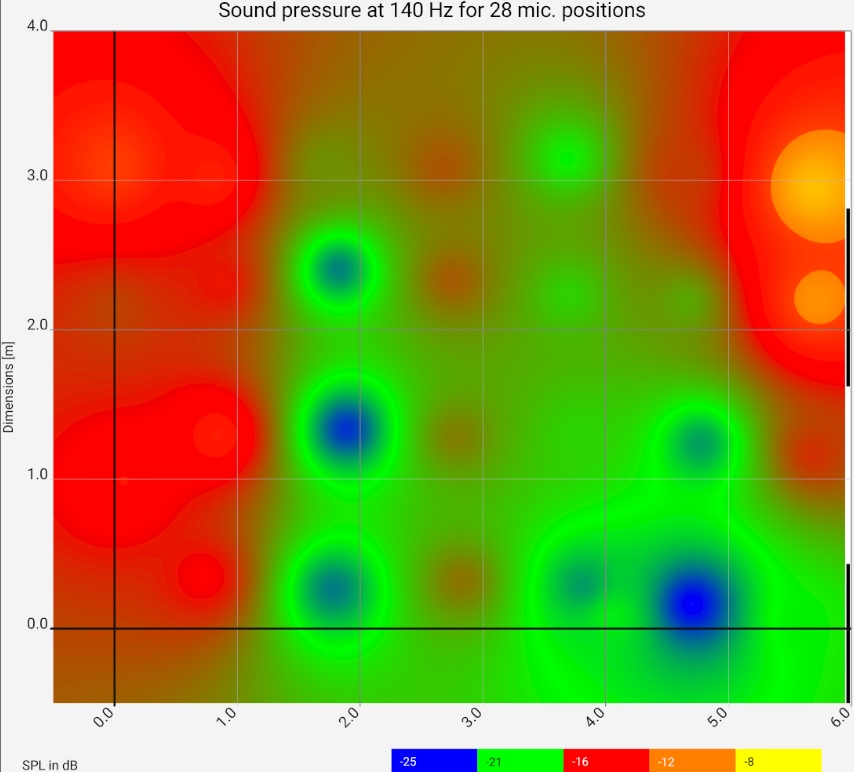
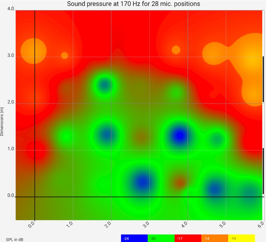 The narrow black/white stripes at the right edge of the picture show the respective wavelength.
It can be seen that the spatial modes build up qualitatively as expected, but their real distribution deviates significantly from a solution of the wave equation in the textbook.
The narrow black/white stripes at the right edge of the picture show the respective wavelength.
It can be seen that the spatial modes build up qualitatively as expected, but their real distribution deviates significantly from a solution of the wave equation in the textbook.
Possibilities for improvement
Only after finding the optimal placement of the speakers and/or the optimal placement of the subwoofer(s) and then determining which modes are still interfering, appropriate absorption material should be ordered. Basically, there are several different ways to get rid of disturbing room modes.- Change of the listening position, i.e. a positioning in the node of the modes so that they are no longer audible.
- Do not excite: The subwoofer is (also) placed near a node of the most interfering mode, thus at least this is not excited.
- Cancellation: Multiple subwoofers are arranged so that the excitations cancel each other out.
- Damping: Narrowband modes (with high Q) can be treated with Helmholz resonators. In forum discussions much more common are so called foil transducers. Porous absorbers are not useful for the very low frequencies discussed here due to space limitations.
- "Separated Volume": Another room connected by an open door acts like a large Helmholz resonator. Also a lowered ceiling with enough space above the second ceiling can act like a damped spring-mass system. The mass of the suspension takes over the role of the air in the neck of the Helmholz resonator, similar to the foil oscillator.
- Sound Processing: Digital sound processing does not eliminate room modes, but can lower their overall level so that at least at a given listening position the desired sum frequency response is achieved.
Personal opinion of the author: To electronically take away the energy of a particularly unpleasant room mode "for the time being", when the next major reconstruction is still in the distant future, is of course worth considering. Otherwise, the sound can become unbearable during some performances. Whether it is then "actually" an excellent room, equipped with the best equipment, does not matter. The sound in an average living room equipped with products from the mass market will be better.
80 to ~300 Hz - Direct reflections
In this frequency range, the wavelengths are smaller than the dimensions of the room (4.3 m at 80 Hz, 1.14 m at 300 Hz), therefore the most important effect can be understood with geometric acoustics: The sound here, after it propagates from the speakers, is absorbed, reflected or scattered by walls and objects - as if the speakers were light sources and the walls (darkened, somewhat cloudy) mirrors. In certain cases, this can actually cause one to perceive the "mirror image" of some instruments in completely the wrong places, e.g. behind a lateral wall.Much more often, however, so-called comb filter effects occur: A sound signal played through a loudspeaker reaches the ear first by a direct path, i.e. the transit time (the time it takes for the signal to travel from the loudspeaker to the ear) corresponds to the distance "loudspeaker to ear" divided by the speed of sound. Depending on the design of the loudspeaker and the condition of the wall, floor and ceiling, reflected signals reach the ear shortly afterwards. For example, if the reflected signal has to travel one meter more, it will reach the ear about 2.9 ms later (1 m / 343 m/s). If we now consider a signal with 343 Hz, the duration of an oscillation (period duration) is also 2.9 ms. With such a signal, the direct part and at the same time the reflected part will arrive at the ear with a delay of one period. Since the delayed signal is "in phase" with the direct signal, both components add up and are perceived as louder together. The same happens with 2, 3, 4... periods, i.e. 2 times, 3 times or 4 times the frequency.
With a signal of half the frequency (171.5 Hz), i.e. twice the period, the opposite will happen: The reflected part and the direct part cancel each other out and the signal heard is attenuated. Something similar happens with 1.5, 2.5, 3.5... periods difference in running time, i.e. 1.5, 2.5 or 3.5 times the frequency.
The following figure illustrates this effect. The user on the right "sees" in addition to the loudspeaker (left, black) a mirror image of the loudspeaker (left, grey) behind, below or above the reflecting surface, here the floor. The longer travel time of the reflected sound is indicated by the red lines, the direct sound is indicated by the green line.
Result:
Possibilities for improvement
Floor reflections occur at very different frequencies depending on the geometry of the speaker and the listening position. As the calculator above shows, the rule of thumb is "first cancellation at 80 - 120 Hz" when, for example, the loudspeaker and ears are about 1.5 m from the ground and 2 m apart. In most cases the frequencies should be much higher. Often any wave-like phenomena in the frequency response in this range are misinterpreted as floor reflections.
Hifi apps therefore allow the user to enter the distances of loudspeaker, floor and listening position and compare the calculated values with the measured frequency spectrum. Only if there are matches with a suspected reflection, countermeasures should be taken. It should be noted that relatively thick damping is required for low frequencies. Even a carpet with a height of 5 cm will only absorb half of the sound at approx. 500 Hz, with a thickness of 2 cm no strong effect can be expected even at 1000 Hz (search engine query: "sound absorption coefficient acoustic foam panel absorber frequency versus thickness", the decisive factor is the ratio of thickness and wavelength, for a rough overview carpet and foam can be seen as comparable).
If an absorber is out of the question, a coffee table or similar may be considered as a diffuser. Or the placement or inclination of the loudspeakers or listening positions can be optimized. Certain loudspeakers avoid reflections by their construction. Without wanting to be insulting: If this is new to you, you should seek professional advice before buying.
Summary
From 200 Hz - directional hearing, integrity and size of the sound image
Reflections and comb filter effects also occur in this range, but the wavelength at 5 kHz, for example, is only 6.9 cm, so that minimal head movements cause strong changes. In fact, our brain can compensate amazingly well for the associated volume changes and they evoke a completely different psychoacoustic effect: from about 200 Hz, indirect reflections create the often desired impression of spaciousness and "envelopment".
As early as 1949, Haas discovered the effect named after him - roughly speaking, that for our sense of orientation it is decisive where the sound comes from first. Reflected sound, which arrives later at the ear (and is naturally no louder than direct sound), "does not count" for locating the sound source.
However, later investigations show that the perception of "stage" and "mirror images of the sound source" is definitely influenced. [Meyer Schroeder 1952] [Lochner Burger 1958] [Olive Toole 1989]. At longer durations, from 80 ms, the "envelopement" builds up, i.e. the impression about the environment in which the musical event takes place. David Griesinger provides material from many years of research work.
Floyd Toole describes further research on human perception depending on the direction of the reflections and the sound material used. The latter (castanets vs. speech) can shift the perception threshold by more than 10 dB. Thus, different recordings should always be used during test listening. The directionality is intuitively clear if we consider that with several equally loud conversations from different directions we can decide which one to follow (party effect). Accordingly, the selection of the mounting locations for the damping elements should also be carefully considered. We can start with the rule of thumb that lateral reflections produce a possibly desirable spatial sound, while reflections from above and below are often undesirable. Presumably, this has to do with the degree of correlation of the signals from both ears: Signals reflected from the floor or ceiling arrive at both ears much more similarly than signals reflected from the side walls. Only the latter create a pleasant enveloping room impression.
Possibilities for improvement
To prevent a single reflection on the wall, floor or ceiling, you can mount a normal (optical) mirror so that you can see the reflection of the sound source at the listening position. An absorber or diffuser must be mounted at this point.Classification
From these findings, the following general principles for automated evaluation are derived: 1) Reflections are not a bad thing: Nearly reflection-free recording studios with near-field monitors are not built for "live" music enjoyment. The automated evaluation in hifi apps therefore allows the definition of thresholds that must first be exceeded before improvement suggestions are initiated. 2) Some reflections are better than others. The subdivision according to durations is one possibility for the first categorization. 3) However, this subdivision must be further specified. Together with the analysis of the (sum) frequency response, usable results are obtained. 4) There are other parameters that can influence these results, ultimately automated measurement cannot replace the work of an experienced sound engineer.
The picture shows a separation between different effects at 200 Hz and 40 ms. Essentially, this is to distinguish between areas with individually audible reflections and modes (below 200 Hz) and areas where diffuse sound determines the listening experience (above 200 Hz). The values are presettings for typical listening rooms, but by no means "natural constants".
fig. 3 Various room acoustics effects sorted by frequency and time. In addition to the frequency f[Hz], the wavelength, half the wavelength (reflections cause amplification at this distance from the wall), a quarter of the wavelength (reflections cause attenuation at this distance from the wall) and the period duration (to compare the magnitude with the running time) are indicated. Effects that are perceived as disturbing are shown in red, effects shown in green or blue are possibly pleasant or neutral in value.
The following table explains the effects in more detail. The values in dB are relative to the direct sound signal. Effects caused by delayed signals above 0 dB are not listed because the reflected signal is normally not stronger than the direct signal. Effects caused by single reflections are only considered up to 10 ms (3.4 m travel distance difference). In typical listening rooms, the first 5 reflections occur in this range. If investigations were made with speech recordings, this is pointed out. In this case, it can be assumed that reflections are perceived earlier and are more disturbing than with music recordings.
| Abbreviation | Effect | Details |
| (SR) | single reflection | The sound impression changes colour due to cancellations and amplifications as described above. In extreme cases, as with WR 2 (see below), a mirror image of the sound source can be heard behind the wall, similar to how the loudspeaker would be seen if an optical mirror were hanging there. |
| ASW (SR) | apparent source width | The apparent width of the sound source, usually the stage. It can differ considerably from the distance between the two front speakers. Reflections from approx. 180 Hz are responsible for this. [Toole], [Griesinger 1999]. Ando, Blauert, Schroeder and other authors propose the interaural cross correlation (IACC) as a measure, i.e. how much the signal of both ears differs. Some authors consider IID (Interaural Intensity Differences) and ITD (Interaural Time Differences) separately for this purpose. In [Sato, Ando] it is shown that IACC and ASW correlate well, and that above 700 Hz for a given angle for reflected sound energy, the lowest IACC occurs simultaneously with the highest ASW. The IACC can again be easily converted to the ratio between lateral and total energy of the first 80ms of the impulse response. |
| COL (SR) | Coloration | The sound is undesirably colored by reflections with an intensity down to -20 dB in some cases [Barron 1971]. |
| ESI | Early spatial Impression Concerns only the first reflections from the front, unlike ENV. | Similar to ASW, ESI can be seen as the ratio of lateral to total sound energy. ASW and ESI are closely related, the differences arising from the direction of the reflected sound and the time profile of intensity. However, IACC cannot be the only effect: Below 300 Hz, there should then be no more spatiality effects, because the wavelength exceeds the ear distance by a multiple. But this is not the case. |
| RM | Room mode | Intensity strongly location-dependent, frequency of maxima/minima location-independent. (See above.) |
| WR 1 (SR) | Low-frequency wall reflection | Often confused with RM. But frequency of maxima/minima is location dependent. Reflections from a wall $n*\lambda/4$ away ($\lambda$ wavelength) cause cancellations ($n$ odd) amplifications ($n$ even). The effect is detectable up to about 120 Hz. So the transit time must be at least half the period of 120 Hz (4 ms), but must not come into the range of multiple reflections. |
| WR 2 (SR) | Low-frequency wall reflection | similar to an optical mirror image, a second sound source becomes perceptible. In [Lochner 1958] this effect is proven for speech at reflections > -5 dB. With longer running times up to approx. 10 ms it weakens at first. (Later, at transit times which do not occur for single reflections in private listening rooms, then it becomes stronger again). |
| FB (SR) | Floor reflection (floor bounce) | Floor reflection calculable by geometric acoustics. (Already described in detail.) |
| SH (SR) | Shift | Can be seen as a weakened version of WR 2. If the reflected signal (for speech playback) exceeds a level of -10dB for delays below 5 ms or -5 dB for 5..10 ms, a shift may become perceptible [Meyer 1952] [Olive 1988]. |
| ENV | Spatial impression (Envelopment) |
Lateral diffuse reflections create a mostly desirable, pleasant enveloping spatial impression for the listener. The listener does not view the music as "through a window", but feels "in" the music.
ENV is treated here the same as LEV (listener envelopment), "spaciousness", BSI (background spatial impression) or SI (spatial impression) [Griesinger][Griesinger 1999].
The representation in green should not hide the fact that there are also disturbing effects with reflections with durations over 50 ms.
Everyone knows such "echo disturbace" effects from announcements in train stations, for example.
Hifi apps do not take these effects into account, as they are below the thresholds measured by [Barron 1971] in common living spaces.
According to [Griesinger 1999], in small listening rooms LEV is generated by interaural fluctuations, which have to be created by the sound engineer during recording.
The loudspeaker / room system works only as a transfer system.
The approaches to measuring how well this works are based on the binaural impulse response are quite different from the older approaches that compare the directions of incidence of different sound components. Ultimately, it is a complex interaction between processing of the recording, loudspeaker and room. Hifi-Apps is therefore limited to a basis on which there is generally consensus: the measurement of the impulse response, from this the determination of the reverberation time, its proportion after a specified time (default 10 ms) and the regularity of the decay behavior. If this is in a harmonic relationship, at least all gross errors that make a good room impression impossible are eliminated. |
Other parameters
For the effects marked in red in Fig. 3, hifi apps calculates scores based on the frequency response and the impulse response. Besides the pattern of the impulse response, the deviations of the frequency responses depending on the listening position, an R/L comparison, etc. are taken into account.In addition, various parameters common in electroacoustics can be output optionally.
- $T_{60}$ ( reverberation time - RT) is the duration in which the sound pressure $p$ drops to the thousandth part when the sound source is suddenly silenced. The corresponding sound pressure level $L_{p}$ then drops by 60 dB.
$$
L_{p}[dB] = 10 \log_{10}\frac{\overline{p}^2}{p_0^2} = 20 \log_{10}\frac{\overline{p} }{p_0 }
$$
For large, reverberant spaces such as churches, the value can be estimated using Sabine's formula:
$T_{60}=0.163 V[m^3]/\sum S_n[m^2]a_n$ where $V$ is room volume and $S_n$ is bounding surfaces, each with absorption coefficient $a_n$.
For typical listening rooms Eyring's formula gives better values, Knudsen's reverberation formula gives the most accurate results.
Sabine's formula is a good basis for estimations:
According to it, the reverberation time is inversely proportional to the absorption coefficient of the insulation material used.
Thus, it provides at least a good orientation: for example, if $T_{60}$ is twice as long as desired, approximately a doubling of the damping material used will be required.
The improvement suggestions of hifi apps are calculated in this way.
Different standards suggest different values for $T_{60}$. The following table provides a brief overview:
The specifications must be met for 200 to 4000 Hz (2500 for N-12A), in other standards the tolerances are larger or these ranges are not specified at all. The threshold for improvement suggestions is preset to 0.6 s for any room in Hifi-Apps.For what Room T_60 IEC 60268-13 Listening tests for loudspeakers in a home environment 20 bis 60 m2 for stereo, 30 to 70 for multichannel 0,3 bis 0,6 s ITU.R Recommendation 1116-1 Assessment of small impairments in audio systems 0,4 to 0,6 s. Target for "natural" sound with increasing room size: $0,25s \cdot \sqrt[3] {V[m^3]/100}$ EBU 3276 Evaluation of programmaterial >40 m2 AES 20 Listening tests (loudspeakers), studio rooms > 20 m2 0,45 s N-12 A Listening tests (General) 60 +/+10 m2 $0,35s \cdot \sqrt {S[m^2]/60}$ - EDT ( early decay time) is the duration in which the sound pressure level has decayed the first 10dB, extrapolated to 60 dB. It plays a more important role for the listening impression than $T_{60}$, because it corresponds better to the subjectively perceived reverberation time: the beginning of the decay curve is perceived best and often the dynamic range of the room does not reach -60 dB. [Fuchs, page 158] explains the decay characteristics of reverberation.
- $F_s$ is the Schröder frequency. It gives an indication for the transition between the dominance of standing waves to the dominance of geometric acoustics. $$ F_s[Hz] = 2000 \sqrt{ \frac{T_{60}[s]}{V[m^3]} } $$ It is indirectly used in the default values for defining the limits of the individual effects, e.g. for the upper frequency up to which room modes are to be detected. The transition is not sharp, in small rooms already at $0.5 F_s$ the statistical behavior typical for high frequencies can be observed. [Skålevik 2011].
- The time constant of a damped harmonic oscillator can be determined from the bandwidth of the resonance. Correspondingly, $T_{60}$ can be determined from the bandwidth $B$ of a room mode (at -3 dB) [Skålevik 2011-2]. $$ B = \frac{\log_e(10^6)}{2 \pi T_{60}} \simeq \frac{2,2}{T_{60}} $$
- The Schröder integral [Schroeder 1965] \begin{align} E(t) &= \int_t^\infty h^2(t) \,dt \\ &= \int_0^\infty h^2(t)\,dt -\int_0^t h^2(t)\,dt \end{align} calculates the amount of energy of the reverberation from time $t$. Practically, only a period of time is integrated in which the background noise is negligible. It is conventional to use the first 10 dB in this backward integrated impulse response for the calculation of the EDT (early decay time) described above.
- The spatial impression $R$ according to [Ballou 2008] is composed of the measured sound energy at the listening position from 25 ms after the source event minus the frontal direct sound from 25 to 80 ms. So at first only the indirect part counts, from 80 ms: $$ R = \log_{10}\left( \frac{(E_{\infty-25})-(E_{80-25}^R)}{E_{25}+(E_{80-25}^R)} \right) $$ Where $E^R$ is the energy component of the sound measured with a directional microphone and $E$ is the component measured with an omnidirectional microphone. The directional microphone had an angle of $\pm 40° $ and is to be directed from the listening position to the sound source. The numbers are ms, for example $E_{\infty-25}$ is the total sound energy minus the sound energy up to 25 ms, i.e. everything measured from 25 ms.
- Mixing Time $t_{mix}$ describes the time of transition between the dominance of single reflections and diffuse late echo, i.e. an ergodic state where the waveform no longer depends on location and time. As a basis for calculation the number of incoming reflections per time $\frac{\,dN}{\,dt}=\frac{4 \pi c^3}{V} t^2$ can be used [Kuttruff][Lindau]. If more than a certain number of reflections per second arrive (Schröder: 1000, Ruback: 4000, Griesinger: 10000) the sound field is perceived as diffuse. The following rule of thumb has been established for this transition $$ t_{mix} [ms] = \sqrt{V [m^3]} $$ $V[m^3]$ is the volume of the listening room in cubic meters. Thus, at a ceiling height of 3 m, 7 ms can be expected for a living room of $15 m^2$ and 12 ms for $50 m^2$. The value can also be determined from the impulse response. [Lindau] compares several methods, Hifi-Apps uses the one of [Huang 2006], since the Computed echo densitiy profile $\eta(t)$ as a "by-product" provides a measure to evaluate the impulse response before $t_{mix}$: $$ \DeclareMathOperator\erfc{erfc} \eta(t) =\frac{1}{2\delta+1} \:\: \frac{1}{\erfc(1/\sqrt{2})} \sum_{\tau=t-\delta}^{t+\delta}{1\{|h(\tau)|>\sigma\}} \\ \sigma= \sqrt{\frac{1}{2\delta+1}\sum_{\tau=t-\delta}^{t+\delta}{\omega(\tau)h^2(\tau)}} $$ Where $\DeclareMathOperator\erfc{erfc} \erfc(1/\sqrt{2}) \simeq 0.3173$. $\delta$ defines a narrow window of the impulse response $h(t)$ (mean set to 0), typically 500 to 2000 samples. The length of the window is thus $2\delta+1$. $\sigma$ is calculated using the windowing function $\omega(t)$, e.g. Hanning or Box. $1\{\cdot\}$ is an indicator function that returns 1 if its argument is TRUE and 0 if it is FALSE. Hifi-Apps uses this algorithm in a slightly modified form: Basis is the logarithmic envelope of the IR, $\sigma$ is determined once in the ergodic part of the IR. This way, the steeply sloping area of direct sound is identified more reliably: There, in addition to the deviation from the Gaussian distribution, the standard deviation is also significantly higher.
- Group delay: The group delay time (GD, symbol $\tau_{gr}$, measured in milliseconds) indicates how long it takes for a certain frequency to be reproduced after the signal has been applied to the input. A "sluggish" woofer can be recognized by a long group delay in the bass range, for example. During playback, drums, for example, could appear "too little impulsive" as a result. Mathematically the group delay results from the negative derivative of the phase $\varphi(\omega)$ of the transfer function $H(j\omega)$ of the system after the angular frequency $\omega$: $$ \tau_{\rm gr}(\omega) = - \frac{\mathrm{d}\varphi(\omega)}{\mathrm{d}\omega}$$ In which cases the GD is audible is controversial. Hifi-Apps therefore use the GD exclusively in connection with listening tests detail.
- Channel equality. For a good stereo image, neither the manufacturing differences between the loudspeakers nor the differences in their positions in the listening room must be too great. The former are often determined electronically by using the voltage at the speaker terminals instead of the microphone signal for the measurement, whereby the amplifier must be connected via a series resistor (Internet search: "Impedance measurement for speakers"). For an accurate measurement with Hifi-Apps, both loudspeakers must change places as close to the millimeter as possible, so that all external conditions are the same. Sound level deviations below 5% are a good value. In practice, it is sometimes astonishing how poorly even trained listeners (want to) perceive significant differences due to defects, incorrect connection or misadjusted crossovers.
For the calculation of the decay times hifi apps use the impulse response. Single peaks are not evaluated. In [Cremer, Müller 1982] it is described that the auditory impression of a peak by a single reflector does not change much if the reflector is divided into several parts with minimally changed propagation time. In the impulse response, however, the one peak becomes 3 smaller peaks close together, so it looks completely different. The ear seems to have a short-term "memory" and "summarizes" the 3 peaks.
Hifi apps divide the impulse response for evaluation into different temporal ranges according to Fig. 3, whereby the defaults for frequency, time and sensitivity can be adjusted. Within these ranges the values are smoothed. Basically, the transitions between these ranges are not to be regarded as sharp: If, for example, dipole speakers are placed too close to a wall, a shift of the source occurs (SH in Fig. 3). It is a matter of judgement at what point it can be called a reflection (WR 2). Probably the individual sense of hearing also plays a role (keyword: HRTF Head-Related Transfer Function ).
The upper and lower cut-off frequencies of the loudspeaker are not specified. They cannot be determined in typical living rooms based on measurements at the listening position In the lower limit range, far too much interference occurs due to room modes and other reflections: Depending on the microphone position, the value can shift by more than an octave - even if the recorded signal has been mathematically processed by smoothing or windowing. In the upper limit the distortions are caused by absorption and the directional characteristic of the tweeters. Above about 4 kHz the built-in microphone is not usable anyway. Hifi apps therefore do not include corresponding values (e.g. when the measured frequency response falls below a certain value) in the ratings. If the values are to be determined nevertheless, near-field measurements (if necessary average values with several loudspeaker setups), measurements outdoors or calculations from the Thiele-Small parameters are suitable.
Possibilities for improvement
In addition to the improvement possibilities described above, hifi apps give further hints based on the impulse responses of the individual speakers at the individual listening positions. The topic is constantly evolving, so only some general statements are made here: In particular, clear weaknesses in channel uniformity and also reverberation times that indicate very little damping can significantly degrade the sound. Both can be easily measured with Hifi-Apps and can often be corrected just as easily. Before taking any measurements, the general instructions for setting up loudspeakers and setting up subwoofers should be taken into account.Literatur
[Ballou 2008] Glenn Ballou: Handbook for Sound Engineers. 2008, Focal Press (Imprint of Elsevier)
[Blauert] Jens Blauert: Spatial Hearing: Psychophysics of Human Sound Localization. MIT Press Ltd; 2 Rev ed edition (11 Oct 1996)
[Barron 1971] Mike Barron: The subjective effects of first reflections in concert halls—The need for lateral reflections. Journal of Sound and Vibration 15(4):475-494 · April 1971
[Bech 1998] Søren Bech: Spatial aspects of reproduced sound in small rooms: The Journal of the Acoustical Society of America 103(1):434-45 · February 1998 Spatial aspects of reproduced sound in small rooms
[Cremer, Müller 1982] Principles and Applications of Room Acoustics, Volume 1, 2. PENINSULA PUB (25 Mar 2016)
[EBU 3276] Listening conditions for the assessment of sound programme material: monophonic and two–channel stereophonic. EBU Tech. 3276 – 2nd edition https://tech.ebu.ch/docs/tech/tech3276.pdf May 1998
[falstad] http://www.falstad.com/modebox/ Ein im Browser lauffähiges Programm zur 3-Dimensionalen Darstellung von Raummoden
[Fuchs, Seite 158] Helmut V. Fuchs: Applied Acoustics: Concepts, Absorbers, and Silencers for Acoustical Comfort and Noise Control. Springer Verlag 2013 ISBN 978-3-642-29366-5 ISBN 978-3-642-29367-2 (eBook)
[Griesinger] David Griesinger: Homepage. http://www.davidgriesinger.com
Griesinger: Spaciousness and envelopment in musical acoustic pdf
[Griesinger 1998] David Griesinger: General overview of spatial impression, envelopment, localization, and externalization. Proceedings of the 15th International AES Conference, Copenhagen, 1998, S 136ff.
[Griesinger 1999] David Griesinger: Objective Measures of Envelopment. AES 16th International Conference on Spatial Sound Reproduction - Apr. 1999 pdf
[Huang 2006] Abel, Jonathan S.; Huang, Patty: A Simple, Robust Measure of Reverberation Echo Density. AES Convention: 121 (October 2006) Paper Number: 6985 Publication Date: October 1, 2006 https://pdfs.semanticscholar.org
[Lindau] Alexander Lindau1, Linda Kosanke1, and Stefan Weinzierl: Perceptual evaluation of physical predictors of the mixing time in binaural room impulse responses. Audio Engineering SocietyConvention Paper Presented at the 128th Convention 2010 May 22–25. impulse_responses.pdf
[Lochner Burger 1958] J.P.A. Lochner, J.F. Burger: The subjective masking of short time delayed echoes by their primary sounds and their contribution to the intelligibility of speech. Acta Acustica united with Acustica 8(1) · January 1958
[Meyer Schroeder 1952] Erwin Meyer, Manfred Schroeder: On the Influence of Reflected Sound on Directional Localization and Loudness of Speech. Wiss. Göttingen, (Math. Phys. Klasse IIa), vol. 6, pp. 31–42 (1952). 1952.
[Olive 1995] Olive, Sean E.; Schuck, Peter L.; Sally, Sharon L.; Bonneville, Marc: The Variability of Loudspeaker Sound Quality Among Four Domestic-Sized Rooms. AES Convention Papers Forum 1995, https://secure.aes.org/forum/pubs/conventions/?elib=7674
[Olive Toole 1989] Sean E. Olive, Floyd E. Toole: The Detection of Reflections in Typical Rooms. AES Convention: 85 (November 1988) Paper Number: 2719 mariobon.com
[Peter 2013] Martin Peter: Visualization of low frequency sound fields in rooms. Inter Noise 2013 Martin_Peter.pdf
[Sato, Ando] Shin-ichi Sato, Yoichi Ando: Apparent Source Width (ASW) of Complex Noises inRelation to the Interaural Cross-correlation Function. Journal of Temporal Design in Architecture and the Environment (2002) Vol. 2; No. 1, P. 29 http://www.jtdweb.org/journal/2002/004_sato.pdf
[Skålevik 2011] Magne Skålevik: Schroeder Frequency Revisited. Forum Acusticum 2011 http://www.akutek.info/Papers/MS_Schroeder_Revisited.pdf
[Skålevik 2011-2] Magne Skålevik: Small room acoustics – the hard case. A paper presented at Forum Acusticum 2011 http://www.akutek.info/Papers/MS_Hard_Case.pdf
[Sereinig] Andrea Sereinig: Specification of a Standardized Listening Room for an Expert Listening Panel. Audio Engineering Project Report Graz, January 2009 PA_Sereinig_A_Standardized_Listening_Room.pdf